An \(\Omega(n^{-1.6342})\) Lower Bound for (Non-Anytime) Gradient Descent
Introduction
Last week, Ma and Chen proved an \(\Omega(n^{-1.932})\) lower bound for gradient descent (GD) under arbitrary predetermined stepsize schedules in smooth convex optimization, and Tsai further improved it to \(\Omega(n^{-1.7321})\) (see his blog post). After multiple rounds of interaction with ChatGPT-5.6 Sol, I obtained the lower bound \(\Omega(n^{-1.6342})\).
We further proved an \(\Omega(n^{-1.2408})\) lower bound for anytime GD in the next blog post.
In the proof, we use the same hard-function family introduced by Ma and Chen. Tsai's blog post gives an insightful explanation of this construction (cf. Tsai's Lemma 6). Our improvement begins after that construction. We estimate the resulting sequence inequality more precisely through term-by-term control of selected long steps instead of compressing those steps into a harmonic mean (cf. Tsai's Lemma 7).
AI Disclosure. This improvement was developed through multiple rounds of interaction with ChatGPT-5.6 Sol. The generated proof was disorganized and difficult to follow. I simplified and rewrote the mathematical presentation.
Problem Setup
Let \(\mathcal F_1(\mathbb R^d)\) be the class of convex \(1\)-smooth functions on \(\mathbb R^d\) whose sets of minimizers are nonempty. Given an integer iteration horizon \(n\ge1\), an initial point \(x_1\in\mathbb R^d\), and a predetermined schedule \(H=(h_1,\ldots,h_n)\in(0,\infty)^n\), GD generates \[ x_{k+1}=x_k-h_k\nabla f(x_k),\qquad 1\le k\le n. \] The schedule may depend on \(n\), but not on \(f\).
Define the worst-case convergence rate by \[ R_n(H):= \sup_{d\in\mathbb N} \sup_{f\in\mathcal F_1(\mathbb R^d)} \sup_{x^\star\in\arg\min f} \sup_{x_1\in\mathbb R^d\setminus\{x^\star\}} \frac{f(x_{n+1})-f(x^\star)} {\frac12\lVert x_1-x^\star\rVert^2}. \]
Our target. Improve Tsai's lower bound \(R_n(H)=\Omega(n^{-1.7321})\) and bring its exponent as close as possible to the \(O(n^{-\log_2(1+\sqrt{2})})\) upper bound of Altschuler and Parrilo.
Main Results
Theorem 1. (Tsai) There exists a universal constant \(c>0\) such that, for every integer \(n\ge1\) and every \(H\in(0,\infty)^n\), \(R_n(H)\ge c n^{-1.7321}\).
We prove the following.
Theorem 2 (Main result). There exists a universal constant \(c>0\) such that, for every integer \(n\ge1\) and every \(H\in(0,\infty)^n\), \(R_n(H)\ge c n^{-1.6342}\).

A two-row diagram uses the same horizontal exponent scale from n to the minus 2 to n to the minus 1. The upper Non-Anytime row shows the lower bounds of Nemirovsky and Yudin, Ma and Chen, Tsai, and This work at exponent 1.6342, followed by the upper bounds of Altschuler and Parrilo and Levitin and Polyak. The lower Anytime row shows the lower bounds of Nemirovsky and Yudin, Tsai and coauthors, and the Next blog at exponent 1.2408, followed by the upper bounds of Zhang and coauthors and Levitin and Polyak.
Up to Lemma 2, we use the hard-function construction of Ma and Chen without modification. This construction gives the product-form lower bound below. Using Tsai's notation, write \(h_{a:b}:=\sum_{k=a}^b h_k\), with an empty sum equal to zero. For an integer \(1\le m\le n\), choose \[ 0<t_1<\cdots<t_m\le n, \qquad h_{t_i}>1, \] set \(t_0=0\), \(t_{m+1}=n+1\), and define \[ S_i:=h_{t_{i-1}+1:t_i-1}, \qquad 1\le i\le m+1. \]
Lemma 2. (cf. Ma and Chen, Theorem 4.1 and Tsai, Lemma 6). For every such selection,
\[ R_n(H)\ge \frac{1}{S_m+h_{t_m}+2S_{m+1}+1} \prod_{i=1}^{m-1} \frac{S_{i+1}+h_{t_{i+1}}} {S_i+h_{t_i}+S_{i+1}+h_{t_{i+1}}} \prod_{i=1}^{m}\frac{h_{t_i}-1}{S_i+1}. \tag{1}\label{eq:hard-product} \]Lemma 2 completes the hard-function construction. From this point on, the rest of the proof amounts to a sequence inequality for the right-hand side of \(\eqref{eq:hard-product}\). Tsai treats the selected long steps collectively through a harmonic mean (cf. Tsai's Lemma 7) and a counting function (cf. Tsai's Lemma 8), which loses information about their individual sizes and chronological pairings. To obtain a sharper estimate, we retain every factor coupling two consecutive selected long steps (Lemma 3) and apply sharper term-by-term estimates (Lemma 4 and Lemma 6).
Reduction to a sequence problem
Lemma 3 (Clean sequence problem). Fix \(\alpha>0\), so the target rate exponent is \(1+\alpha\). For \(w,z,x,y>0\), define
\[ K_{w,z}(x,y):= \frac{\sqrt{xy}\,(w+z+x+y)}{\sqrt{wz(w+x)(z+y)}} \tag{2}\label{eq:kernel} . \]To prove \(R_n(H)\ge c_\alpha(n+1)^{-(1+\alpha)}\) for every \(n\) and \(H\), it is enough to find a constant \(C_\alpha<\infty\), depending only on \(\alpha\), such that the following holds for every integer \(q\ge2\). Given positive sequences \(x_1,\ldots,x_q\) and \(\omega_1,\ldots,\omega_q\), write \(\omega_1^\downarrow\ge\cdots\ge\omega_q^\downarrow\) for the decreasing rearrangement of \((\omega_i)\). If
\[ \sum_{i=1}^q x_i<q, \qquad \sum_{s=m+1}^q \omega_s^\downarrow \ge q\left[\left(\frac qm\right)^\alpha-1\right], \qquad 1\le m<q. \tag{3}\label{eq:sequence-constraints} \]then
\[ E_{\mathrm{end}} \prod_{i=1}^{q-1}K_{\omega_i,\omega_{i+1}}(x_i,x_{i+1}) \le C_\alpha, \tag{4}\label{eq:sequence-bound} \]where
\[ E_{\mathrm{end}}:= \sqrt{x_1x_q}\sqrt{\frac{1+x_1/\omega_1}{1+x_q/\omega_q}} \left[1+\frac{x_q+2\left(q-\sum_{i=1}^q x_i\right)}{\omega_q}\right]. \tag{5}\label{eq:endpoint-factor} \]Full proof
Suppose \(\eqref{eq:sequence-constraints}\) implies \(\eqref{eq:sequence-bound}\) with a constant \(C_\alpha\) uniform over \(q\ge2\). Fix \(n\ge1\) and a schedule \(H=(h_1,\ldots,h_n)\). Let \(r:=\#\{k:h_k>1\}\) and \(B:=1+\sum_{k=1}^n\min\{h_k,1\}\).
Case 1: \(r\ge1\). List the positive numbers \(h_k-1\) as \(a_1\ge\cdots\ge a_r>0\), and define \(D_s:=B+\sum_{\ell=s+1}^r a_\ell\) for \(1\le s\le r\). Then \(1+\sum_{k=1}^n h_k=B+\sum_{\ell=1}^r a_\ell\) and \(D_r=B\). Choose \[ q\in\operatorname*{arg\,min}_{1\le s\le r}D_s s^\alpha. \] Thus \(D_q q^\alpha\le D_s s^\alpha\) for every \(1\le s\le r\).
We first treat the general case \(q\ge2\), which is the case where condition \(\eqref{eq:sequence-constraints}\) is needed.
Case 1a: \(q\ge2\). Let \(t_1<\cdots<t_q\) be the indices of the \(q\) largest positive excesses \(h_k-1\). With \(S_1,\ldots,S_{q+1}\) defined as in Lemma 2, the intervals defining these sums partition the indices outside \(\{t_1,\ldots,t_q\}\). Therefore \[ \sum_{i=1}^{q+1}(S_i+1) =q+1+\sum_{k\notin\{t_1,\ldots,t_q\}}h_k =D_q. \] Define \[ x_i=\frac{q(S_i+1)}{D_q}, \qquad \omega_i=\frac{q(h_{t_i}-1)}{D_q}. \] Then \[ \sum_{i=1}^q x_i =\frac q{D_q}\sum_{i=1}^q(S_i+1) =q-\frac{q(S_{q+1}+1)}{D_q} <q. \] Moreover, \(\omega_s^\downarrow=qa_s/D_q\) for \(1\le s\le q\). For every \(1\le m<q\), the minimizing property of \(q\), namely \(D_q q^\alpha\le D_m m^\alpha\), gives \[ 1+\frac1q\sum_{s=m+1}^q\omega_s^\downarrow =1+\frac{\sum_{s=m+1}^q a_s}{D_q} =\frac{D_m}{D_q} \ge\left(\frac qm\right)^\alpha. \] Thus \(x_i,\omega_i\) satisfy \(\eqref{eq:sequence-constraints}\).
Let \(G\) be the right-hand side of \(\eqref{eq:hard-product}\), with \(m=q\) and the indices chosen above. Lemma 2 gives \(R_n(H)\ge G\), and substitution yields \[ G^{-1} =\frac{D_q}{q}\sqrt{x_1x_q} \sqrt{\frac{1+x_1/\omega_1}{1+x_q/\omega_q}} \left[ 1+\frac{x_q+2(q-\sum_{i=1}^q x_i)-q/D_q}{\omega_q} \right] \prod_{i=1}^{q-1} K_{\omega_i,\omega_{i+1}}(x_i,x_{i+1}). \] The bracket is positive, since \[ 1+\frac{x_q+2(q-\sum_{i=1}^q x_i)-q/D_q}{\omega_q} =\frac{S_q+h_{t_q}+2S_{q+1}+1}{h_{t_q}-1}>0. \] Replacing \(-q/D_q\) by \(0\) increases the bracket. Therefore \(\eqref{eq:sequence-bound}\) gives \[ G^{-1} \le \frac{D_q}{q} E_{\mathrm{end}} \prod_{i=1}^{q-1}K_{\omega_i,\omega_{i+1}}(x_i,x_{i+1}) \le\frac{D_q}{q}C_\alpha, \qquad R_n(H)\ge G\ge\frac{q}{C_\alpha D_q}. \] Since \(D_q q^\alpha\le D_r r^\alpha=Br^\alpha\), we obtain \[ R_n(H) \ge\frac{q}{C_\alpha D_q} \ge\frac{q^{1+\alpha}}{C_\alpha Br^\alpha} \ge\frac1{C_\alpha B(r+1)^\alpha}. \]
It remains to treat the boundary cases outside Case 1a. For these cases, we use the following Huber loss to construct a lower bound.
Set \(\delta:=(1+2\sum_{k=1}^n h_k)^{-1}\), and consider the one-dimensional convex, \(1\)-smooth Huber function \[ f_\delta(x):= \begin{cases} x^2/2,& |x|\le\delta,\\ \delta|x|-\delta^2/2,& |x|>\delta. \end{cases} \] Let \(\xi_1,\ldots,\xi_{n+1}\) be the GD iterates on \(f_\delta\) generated by \(H\), with \(\xi_1:=1\) and \(\xi_{k+1}:=\xi_k-h_k f_\delta'(\xi_k)\) for \(1\le k\le n\). An induction gives \[ \xi_k =1-\delta\sum_{j=1}^{k-1}h_j \ge 1-\delta\sum_{j=1}^n h_j >\delta, \qquad 1\le k\le n+1. \] Hence every iterate lies in the region \(x>\delta\), where \(f_\delta'(x)=\delta\). The minimizer is \(0\), and the choice of \(\delta\) gives \(R_n(H)\ge2f_\delta(\xi_{n+1})=\delta\).
Case 1b: \(q=1\). Since \(D_1+a_1=1+\sum_{k=1}^n h_k\), the Huber bound gives \(R_n(H)\ge[2(D_1+a_1)-1]^{-1}\). If \(a_1\le D_1\), this is at least \(1/(4D_1)\). If \(a_1>D_1\), choose an index \(t\) with \(h_t-1=a_1\), and apply Lemma 2 with \(m=1\) and \(t_1=t\). Then \(D_1=(S_1+1)+(S_2+1)\), and \((S_1+1)+a_1+2(S_2+1)-1<a_1+2D_1<3a_1\). Lemma 2 therefore gives \[ R_n(H) \ge\frac{a_1}{(S_1+1)(S_1+a_1+2S_2+2)} >\frac1{3(S_1+1)} \ge\frac1{3D_1} >\frac1{4D_1}. \] Thus \(R_n(H)\ge1/(4D_1)\) in either subcase. Using the minimizing property with \(s=r\), we obtain \(D_1\le D_r r^\alpha=Br^\alpha\), and hence \[ R_n(H)\ge\frac1{4B(r+1)^\alpha}. \]
Case 2: \(r=0\). Here \(h_k\le1\) for every \(k\), so \(B=1+\sum_{k=1}^n h_k\) and \(\delta=(2B-1)^{-1}\). The Huber bound gives \(R_n(H)\ge(2B-1)^{-1}\ge(2B)^{-1}\).
Since \(B\le n+1\) and \(r+1\le n+1\), these estimates give \[ R_n(H)\ge c_\alpha(n+1)^{-(1+\alpha)}, \qquad c_\alpha:=\min\{C_\alpha^{-1},1/4\}. \]
Eliminating the variables \(x_i\)
To make \(\eqref{eq:sequence-bound}\) more tractable, we first eliminate the variables \(x_i\). For a parameter \(\lambda>0\), to be chosen later, define \[ \Gamma_\lambda(w,z) := \sup_{x,y>0} \left\{ \log K_{w,z}(x,y)-\lambda(x+y) \right\}. \tag{6}\label{eq:gamma-definition} \] By definition, for every \(w,z,x,y>0\), \[ \log K_{w,z}(x,y) \le \lambda(x+y)+\Gamma_\lambda(w,z). \tag{7}\label{eq:gamma-envelope} \] Lemma 4 applies \(\eqref{eq:gamma-envelope}\) to each \(K_{\omega_i,\omega_{i+1}}(x_i,x_{i+1})\), \(1\le i<q\), and eliminates the variables \(x_i\) using the condition \(\sum_{i=1}^q x_i\le q\).
Lemma 4. Fix \(\alpha,\lambda>0\). There is a constant \(C_{\alpha,\lambda}<\infty\) such that, for every integer \(q\ge2\), every pair of positive sequences \((x_i)_{i=1}^q\) and \((\omega_i)_{i=1}^q\) satisfying \(\eqref{eq:sequence-constraints}\) obeys
\[ E_{\mathrm{end}} \prod_{i=1}^{q-1}K_{\omega_i,\omega_{i+1}}(x_i,x_{i+1}) \le C_{\alpha,\lambda} \exp\!\left\{ 2\lambda q+ \sum_{i=1}^{q-1}\Gamma_\lambda(\omega_i,\omega_{i+1}) \right\}. \tag{8}\label{eq:envelope-reduction} \]Full proof
Set \(\Delta:=q-\sum_{i=1}^q x_i>0\). Applying \(\eqref{eq:gamma-envelope}\) to \(K_{\omega_i,\omega_{i+1}}(x_i,x_{i+1})\) for \(1\le i<q\) and summing gives \[ \log\prod_{i=1}^{q-1}K_{\omega_i,\omega_{i+1}}(x_i,x_{i+1}) \le\lambda\sum_{i=1}^{q-1}(x_i+x_{i+1}) +\sum_{i=1}^{q-1}\Gamma_\lambda(\omega_i,\omega_{i+1}). \] Since \(\sum_{i=1}^{q-1}(x_i+x_{i+1}) =2\sum_{i=1}^q x_i-x_1-x_q=2q-(2\Delta+x_1+x_q)\), we obtain \[ \begin{aligned} E_{\mathrm{end}}\prod_{i=1}^{q-1}K_{\omega_i,\omega_{i+1}}(x_i,x_{i+1}) &\le \exp\!\left\{ 2\lambda q+ \sum_{i=1}^{q-1}\Gamma_\lambda(\omega_i,\omega_{i+1}) \right\}\\ &\qquad{}\times E_{\mathrm{end}}e^{-\lambda(2\Delta+x_1+x_q)}. \end{aligned} \] It remains to bound \(E_{\mathrm{end}}e^{-\lambda(2\Delta+x_1+x_q)}\) independently of \(q\), \((x_i)_{i=1}^q\), and \((\omega_i)_{i=1}^q\).
Taking \(m=q-1\) in \(\eqref{eq:sequence-constraints}\) yields \[ \min_{1\le i\le q}\omega_i =\omega_q^\downarrow \ge q\left[\left(\frac q{q-1}\right)^\alpha-1\right] \ge\alpha q\log\frac q{q-1} \ge\alpha. \] Here the last two inequalities use \(e^u-1\ge u\) and \(\log(1+t)\ge t/(1+t)\). In particular, \(\omega_1,\omega_q\ge\alpha\). Using this in \(\eqref{eq:endpoint-factor}\) and writing \(T:=x_1+x_q+\Delta\), we directly obtain \[ E_{\mathrm{end}}e^{-\lambda(2\Delta+x_1+x_q)} \le C_\alpha(1+T)^{5/2}e^{-\lambda T} \le C_\alpha\sup_{t\ge0}(1+t)^{5/2}e^{-\lambda t} =:C_{\alpha,\lambda}<\infty. \] This proves \(\eqref{eq:envelope-reduction}\).
Basic properties of \(\Gamma_\lambda\)
Lemma 5. For every \(\lambda>0\), \(\Gamma_\lambda\) has the following properties.
(1) Smoothness. For every \(w,z>0\), the supremum in \(\eqref{eq:gamma-definition}\) is attained at a unique pair \((x_\lambda(w,z),y_\lambda(w,z))\in(0,\infty)^2\). The optimizer map \((w,z)\mapsto(x_\lambda(w,z),y_\lambda(w,z))\) and \(\Gamma_\lambda\) are \(C^\infty\) on \((0,\infty)^2\).
(2) Symmetry. \(\Gamma_\lambda(w,z)=\Gamma_\lambda(z,w)\).
(3) Joint convexity. The map \((w,z)\mapsto\Gamma_\lambda(w,z)\) is jointly convex on \((0,\infty)^2\).
(4) Decreasing in each coordinate. \(\Gamma_\lambda\) is strictly decreasing in each coordinate.
(5) Strict submodularity. \[ \partial_{wz}^2\Gamma_\lambda(w,z)<0. \tag{9}\label{eq:submodularity} \]
Full proof
(1) Smoothness. Let \(F_{w,z}(x,y):=\log K_{w,z}(x,y)-\lambda(x+y)\). For fixed \(w,z>0\), \(F_{w,z}(x,y)\to-\infty\) as \(x\downarrow0\), \(y\downarrow0\), or \(x+y\to\infty\). Hence it attains its maximum at an interior point. Write \(A:=w+x\), \(B:=z+y\), and \(\Sigma:=A+B\). For every nonzero direction \((a,b)\), \[ D^2_{x,y}F_{w,z}[(a,b)]^2 =-\frac{a^2}{2x^2}-\frac{b^2}{2y^2} -\frac{(a+b)^2}{\Sigma^2} +\frac{a^2}{2A^2}+\frac{b^2}{2B^2}<0. \] Thus the maximizer is unique. Fix \((w_0,z_0)\), and let \((x_0,y_0)\) be its maximizer. The Jacobian in \((x,y)\) of the first-order condition \(\nabla_{x,y}F_{w,z}(x,y)=0\) is the invertible Hessian above. The implicit function theorem therefore gives a neighborhood \(U\) of \((w_0,z_0)\) and a \(C^\infty\) solution \((x(w,z),y(w,z))\) of this system on \(U\). For every \((w,z)\in U\), strict concavity makes this critical point the unique global maximizer. Hence the local solution maps obtained from different base points agree on their overlaps. Since \((w_0,z_0)\) was arbitrary, \((w,z)\mapsto(x_\lambda(w,z),y_\lambda(w,z))\) is \(C^\infty\) on \((0,\infty)^2\). Substitution into \(F_{w,z}\) proves the same for \(\Gamma_\lambda\).
(2) Symmetry. The definition \(\eqref{eq:gamma-definition}\) is invariant under \((w,x)\leftrightarrow(z,y)\), which proves Property (2).
(3) Joint convexity. For fixed \(x,y\), put \(A:=w+x\) and \(B:=z+y\). The Hessian in \((w,z)\) has quadratic form \[ \frac{a^2}{2w^2}+\frac{a^2}{2A^2} +\frac{b^2}{2z^2}+\frac{b^2}{2B^2} -\frac{(a+b)^2}{(A+B)^2}\ge0. \] The first four terms dominate \(a^2/A^2+b^2/B^2\), which is at least \((a+b)^2/(A+B)^2\) by Cauchy–Schwarz. Taking the supremum in \(\eqref{eq:gamma-definition}\) preserves convexity, proving Property (3).
(4) Decreasing in each coordinate. Write \(x_\ast:=x_\lambda(w,z)\), \(y_\ast:=y_\lambda(w,z)\), and set \(A:=w+x_\ast\), \(B:=z+y_\ast\), and \(\Sigma:=A+B\). The chain rule and the first-order conditions give \[ \begin{aligned} \partial_w\Gamma_\lambda &=\partial_wF_{w,z} +\partial_xF_{w,z}\,\partial_wx_\ast +\partial_yF_{w,z}\,\partial_wy_\ast\\ &=\partial_wF_{w,z} =\frac1\Sigma-\frac1{2w}-\frac1{2A}. \end{aligned} \] Equivalently, \[ -\partial_w\Gamma_\lambda =\frac{x_\ast}{2wA}+\frac{B}{A\Sigma}>0, \] and similarly in \(z\). This proves Property (4).
(5) Strict submodularity. With the notation from Property (4), the first-order conditions imply \[ \lambda-\frac1\Sigma =\frac{w}{2x_\ast A} =\frac{z}{2y_\ast B}. \] Thus \[ \tau_\ast:=\frac{x_\ast A}{w} =\frac{y_\ast B}{z}>0. \] For \(u,\tau>0\), set \[ A_u(\tau):=\frac{u+\sqrt{u^2+4u\tau}}2. \] Then \(A=A_w(\tau_\ast)\), \(B=A_z(\tau_\ast)\), and \[ g(\tau_\ast;w,z)=0, \qquad g(\tau;w,z):= \frac1{2\tau}+\frac1{A_w(\tau)+A_z(\tau)}-\lambda. \] The explicit formula for \(A_u\) shows that it increases in both arguments, so \(\partial_\tau g<0\) and \(\partial_zg<0\). Implicit differentiation now gives \(\partial_z\tau_\ast=-(\partial_zg)/(\partial_\tau g)<0\). Moreover, \[ \Sigma=\left(\lambda-\frac1{2\tau_\ast}\right)^{-1}, \qquad A=A_w(\tau_\ast). \] Since \(d\Sigma/d\tau=-\Sigma^2/(2\tau^2)<0\), we have \(\partial_z\Sigma>0\) and \(\partial_z A=A_w'(\tau_\ast)\partial_z\tau_\ast<0\). Differentiating the formula for \(\partial_w\Gamma_\lambda\) gives \[ \partial_{wz}^2\Gamma_\lambda = -\frac{\partial_z\Sigma}{\Sigma^2} +\frac{\partial_z A}{2A^2}<0, \] proving Property (5).
Upper bounding \(\sum_{i=1}^{q-1}\Gamma_\lambda(\omega_i,\omega_{i+1})\)
Recall from Lemma 3 that \(\omega_1^\downarrow\ge\cdots\ge\omega_q^\downarrow\) is the decreasing rearrangement of \(\omega_1,\ldots,\omega_q\).
For a positive vector \(v=(v_1,\ldots,v_N)\) and \(0\le k\le\lfloor N/2\rfloor\), let \(\mathcal M_k(N)\) be the set of all collections of \(k\) disjoint unordered pairs from \(\{1,\ldots,N\}\). Define \[ \Phi_{k,\lambda}(v_1,\ldots,v_N) := \max_{M\in\mathcal M_k(N)} \sum_{\{a,b\}\in M}\Gamma_\lambda(v_a,v_b). \] Thus \(\Phi_{k,\lambda}(v)\) is the maximum sum over all collections of \(k\) disjoint pairs of coordinates of \(v\). We set \(\Phi_{0,\lambda}=0\).
Splitting the terms in \(\sum_{i=1}^{q-1}\Gamma_\lambda(\omega_i,\omega_{i+1})\) according to whether \(i\) is odd or even gives two matchings.
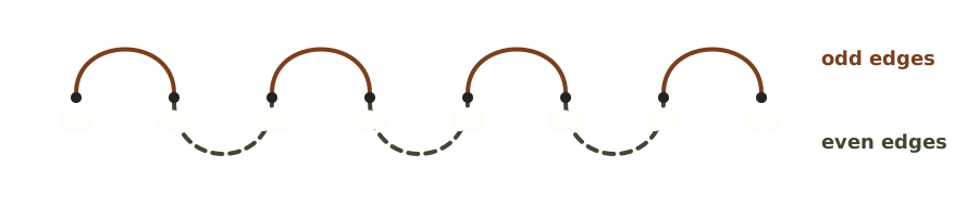
Set \(k_q:=\lfloor(q-1)/2\rfloor\). By the coordinatewise-decreasing property in Lemma 5(4), \(\Gamma_\lambda(\omega_i,\omega_j)\le\Gamma_\lambda(\alpha,\alpha)\), since \(\eqref{eq:sequence-constraints}\) with \(m=q-1\) gives \(\omega_i,\omega_j\ge\alpha\). Splitting the sum into these two matchings and treating the one possible deleted pair with the bound above gives \[ \sum_{i=1}^{q-1}\Gamma_\lambda(\omega_i,\omega_{i+1}) \le 2\Phi_{k_q,\lambda} (\omega_q^\downarrow,\ldots,\omega_2^\downarrow) +C_{\alpha,\lambda}. \tag{10}\label{eq:parity-bound} \] See the full proof for details.
We now bound \(\Phi_{k_q,\lambda}\) through two finer reductions, using the properties of \(\Gamma_\lambda\) established in Lemma 5.
Step 1. Majorization
For \(2\le s\le q\), define
\[ \bar w_s^{(q)} := q^{1+\alpha}\bigl((s-1)^{-\alpha}-s^{-\alpha}\bigr), \qquad 2\le s\le q. \tag{11}\label{eq:reference-weights} \]Their tails satisfy \[ \sum_{s=m+1}^q\bar w_s^{(q)} =q\left[\left(\frac qm\right)^\alpha-1\right]. \] Together with \(\eqref{eq:sequence-constraints}\), this gives \[ \sum_{s=m+1}^q\omega_s^\downarrow \ge \sum_{s=m+1}^q\bar w_s^{(q)}, \qquad 1\le m<q. \] Because \(\Gamma_\lambda\) is symmetric, jointly convex, and coordinatewise decreasing (Lemma 5), the function \(\Phi_{k,\lambda}\) is symmetric, convex, and coordinatewise decreasing as well. The tail comparison above therefore gives \[ \Phi_{k_q,\lambda} (\omega_q^\downarrow,\ldots,\omega_2^\downarrow) \le \Phi_{k_q,\lambda} (\bar w_q^{(q)},\ldots,\bar w_2^{(q)}). \tag{12}\label{eq:majorization-comparison} \]
Step 2. Identify the maximizing pairing
Let \(0<v_1\le\cdots\le v_N\) and \(0\le k\le\lfloor N/2\rfloor\). Since \(\Gamma_\lambda\) decreases in each coordinate, a maximizing matching in \(\Phi_{k,\lambda}(v)\) may be chosen to use the \(2k\) smallest entries. Symmetry and strict submodularity imply that a maximizing matching pairs \(v_j\) with \(v_{2k+1-j}\). \[ \Phi_{k,\lambda}(v_1,\ldots,v_N) = \sum_{j=1}^k \Gamma_\lambda(v_j,v_{2k+1-j}). \tag{13}\label{eq:maximizing-pairing} \] The numbers in \(\eqref{eq:reference-weights}\) satisfy \(\bar w_q^{(q)}\le\cdots\le\bar w_2^{(q)}\), so \(\eqref{eq:maximizing-pairing}\) applies directly to \((\bar w_q^{(q)},\ldots,\bar w_2^{(q)})\). In particular,
\[ \Phi_{k_q,\lambda}(\bar w_q^{(q)},\ldots,\bar w_2^{(q)}) =\sum_{j=1}^{k_q} \Gamma_\lambda(\bar w_{q+1-j}^{(q)},\bar w_{q-2k_q+j}^{(q)}). \tag{14}\label{eq:reference-pairing} \]By the mean value theorem, for every \(2\le s\le q\), there is \(\theta_s\in(s-1,s)\) such that
\[ \bar w_s^{(q)}=W_\alpha(\theta_s/q), \qquad W_\alpha(t):=\alpha t^{-1-\alpha},\quad 0<t\le1. \tag{15}\label{eq:mean-value-profile} \]By Lemma 6.2, replacing the mean-value points in \(\eqref{eq:reference-pairing}\) by the mesh points changes the sum by \(O_{\alpha,\lambda}(1)\), and the uncovered part of \([0,1/2]\) contributes another \(O_{\alpha,\lambda}(1)\). Therefore
\[ \sum_{j=1}^{k_q} \Gamma_\lambda(\bar w_{q+1-j}^{(q)},\bar w_{q-2k_q+j}^{(q)}) \le q\int_0^{1/2} \Gamma_\lambda\bigl(W_\alpha(t),W_\alpha(1-t)\bigr)\,dt +C_{\alpha,\lambda}. \]Combining this with \(\eqref{eq:parity-bound}\), \(\eqref{eq:majorization-comparison}\), and \(\eqref{eq:reference-pairing}\) gives the following lemma.
Lemma 6. Fix \(\alpha,\lambda>0\). There is a constant \(C_{\alpha,\lambda}<\infty\) such that, for every integer \(q\ge2\) and every positive sequence \(\omega_1,\ldots,\omega_q\) satisfying the tail condition in \(\eqref{eq:sequence-constraints}\),
\[ \sum_{i=1}^{q-1}\Gamma_\lambda(\omega_i,\omega_{i+1}) \le 2q\int_0^{1/2} \Gamma_\lambda\bigl(W_\alpha(t),W_\alpha(1-t)\bigr)\,dt +C_{\alpha,\lambda}. \tag{16}\label{eq:path-estimate} \]Full proof
(1) Proof of \(\eqref{eq:parity-bound}\). We treat odd and even \(q\) separately. Put \(k_q=\lfloor(q-1)/2\rfloor\), and choose an index \(i_\star\) such that \(\omega_{i_\star}=\omega_1^\downarrow\). If \(q\) is odd, each parity matching has \(k_q\) pairs and leaves one index unused. If \(i_\star\) is matched, replace it by the unused index. The unused coordinate has no larger value, so Lemma 5(4) shows that the sum cannot decrease.
If \(q\) is even, the same replacement applies to the matching with \(k_q\) pairs. The other matching is perfect. Delete its unique pair containing \(i_\star\). Each remaining matching then has \(k_q\) pairs drawn from \((\omega_q^\downarrow,\ldots,\omega_2^\downarrow)\), and is therefore bounded by \(\Phi_{k_q,\lambda}(\omega_q^\downarrow,\ldots,\omega_2^\downarrow)\). Taking \(m=q-1\) in \(\eqref{eq:sequence-constraints}\) gives \[ \omega_q^\downarrow \ge q\left[\left(\frac q{q-1}\right)^\alpha-1\right] \ge q\alpha\log\frac q{q-1} \ge\alpha, \] where the last step uses \(\log(1+t)\ge t/(1+t)\). Hence every \(\omega_i\ge\alpha\), and Lemma 5(4) gives \(\Gamma_\lambda(\omega_i,\omega_j)\le \Gamma_\lambda(\alpha,\alpha)\). In particular, the pair deleted in the even case is bounded by \(\max\{0,\Gamma_\lambda(\alpha,\alpha)\}\). This proves \(\eqref{eq:parity-bound}\).
(2) Proof of Step 1. Majorization. For a fixed matching, the sum of its \(\Gamma_\lambda\)-terms is convex and coordinatewise decreasing. Taking the maximum over all matchings preserves both properties, and permuting the coordinates only permutes the matchings. Hence \(\Phi_{k,\lambda}\) is symmetric, convex, and coordinatewise decreasing.
Lemma 6.1. Let \(F:(0,\infty)^N\to\mathbb R\) be symmetric, convex, and coordinatewise decreasing. If \(a_1\le\cdots\le a_N\), \(b_1\le\cdots\le b_N\), and \(\sum_{i=1}^{\ell}a_i\ge\sum_{i=1}^{\ell}b_i\) for every \(1\le\ell\le N\), then \(F(a)\le F(b)\).
Proof. In the application below, \(F=\Phi_{k_q,\lambda}\). Although \(\Gamma_\lambda\) is smooth, \(F\) is a maximum over matchings and need not be differentiable when several matchings tie. Choose a subgradient \(g\in\partial F(a)\), meaning \(F(y)\ge F(a)+g\cdot(y-a)\) for every \(y\). It exists because \(F\) is finite and convex on \((0,\infty)^N\).
Average \(g\) over the permutations that leave \(a\) fixed; the average is still a subgradient at \(a\). Applying its defining inequality after swapping two unequal coordinates of \(a\), and using symmetry of \(F\), gives \(g_1\le\cdots\le g_N\). Coordinatewise decrease gives \(g_i\le0\). With \(D_\ell:=\sum_{i=1}^{\ell}(b_i-a_i)\le0\), summation by parts yields \[ g\cdot(b-a) =g_ND_N+ \sum_{\ell=1}^{N-1}(g_\ell-g_{\ell+1})D_\ell \ge0. \] Thus \(F(b)\ge F(a)+g\cdot(b-a)\ge F(a)\). \(\square\)
We apply Lemma 6.1 to \(F=\Phi_{k_q,\lambda}\). Formula \(\eqref{eq:reference-weights}\) can be written as \(\bar w_s^{(q)}=q^{1+\alpha}\int_{s-1}^{s}\alpha u^{-1-\alpha}\,du\). Since the integrand decreases, \(\bar w_q^{(q)}\le\cdots\le\bar w_2^{(q)}\), and for \(1\le m<q\), \[ \sum_{s=m+1}^q\bar w_s^{(q)} =q^{1+\alpha}\int_m^q\alpha u^{-1-\alpha}\,du =q\left[\left(\frac qm\right)^\alpha-1\right]. \] Setting \(m=q-\ell\) in \(\eqref{eq:sequence-constraints}\) gives, for \(1\le\ell\le q-1\), \[ \sum_{i=1}^{\ell}\omega_{q+1-i}^\downarrow \ge\sum_{i=1}^{\ell}\bar w_{q+1-i}^{(q)}. \] Lemma 6.1, applied to \(a=(\omega_q^\downarrow,\ldots,\omega_2^\downarrow)\) and \(b=(\bar w_q^{(q)},\ldots,\bar w_2^{(q)})\), now gives \[ \Phi_{k_q,\lambda} (\omega_q^\downarrow,\ldots,\omega_2^\downarrow) \le \Phi_{k_q,\lambda} (\bar w_q^{(q)},\ldots,\bar w_2^{(q)}), \] which is \(\eqref{eq:majorization-comparison}\).
(3) Proof of Step 2. Identify the maximizing pairing. For \(0<a\le b\le c\le d\), symmetry and strict submodularity give \[ \begin{aligned} \Gamma_\lambda(a,d)+\Gamma_\lambda(b,c) &\ge\Gamma_\lambda(a,c)+\Gamma_\lambda(b,d),\\ \Gamma_\lambda(a,d)+\Gamma_\lambda(b,c) &\ge\Gamma_\lambda(a,b)+\Gamma_\lambda(c,d). \end{aligned} \] Now let \(0<v_1\le\cdots\le v_N\). Because \(\Gamma_\lambda\) decreases in each coordinate, a maximizing matching uses the \(2k\) smallest coordinates. If the smallest selected value \(v_1\) is not paired with the largest selected value \(v_{2k}\), exchange the partners of their two pairs. The two displayed inequalities show that the total cannot decrease. Fix the pair \((v_1,v_{2k})\) and repeat with the remaining values. This gives the pairing in \(\eqref{eq:maximizing-pairing}\).
(4) Compare the finite sum with the integral. For every \(2\le s\le q\), let \(\theta_s\in(s-1,s)\) be the point in \(\eqref{eq:mean-value-profile}\). Define \[ G(t,v):=\Gamma_\lambda(W_\alpha(t),W_\alpha(v)), \qquad 0<t\le1,\quad \frac12\le v\le1. \]
Lemma 6.2 (A uniform Lipschitz bound near \(t=0\)). For fixed \(\alpha,\lambda>0\), \(G\) has a Lipschitz extension to \([0,1]\times[1/2,1]\).
Proof. Put \(w:=W_\alpha(t)\), \(z:=W_\alpha(v)\), and let \((x_\ast,y_\ast)\) be the optimizer in \(\eqref{eq:gamma-definition}\). The first-order relations used in Lemma 5(5) give \[ \tau_\ast :=\frac{x_\ast(w+x_\ast)}w =\frac{y_\ast(z+y_\ast)}z, \qquad \lambda =\frac1{2\tau_\ast} +\frac1{w+x_\ast+z+y_\ast}. \] Since \(\alpha\le z\le\alpha2^{1+\alpha}\) and \(z+y_\ast\ge\sqrt{z\tau_\ast}\), we have \[ \lambda \le\frac1{2\tau_\ast} +\frac1{\sqrt{\alpha\tau_\ast}}. \] The right-hand side tends to \(0\) as \(\tau_\ast\to\infty\), so \(\tau_\ast\le C_{\alpha,\lambda}\). In particular, \(x_\ast,y_\ast\le\tau_\ast\).
The bounds on \(z\) and \(y_\ast\) give \(B:=z+y_\ast\le\alpha2^{1+\alpha}+C_{\alpha,\lambda}\), while \(A:=w+x_\ast\ge w\) and \(\Sigma:=A+B\ge w\). The derivative identity in Lemma 5(4) therefore gives \[ |\partial_w\Gamma_\lambda(w,z)| \le C_{\alpha,\lambda}w^{-2}. \] Its symmetric version is \[ -\partial_z\Gamma_\lambda(w,z) =\frac{y_\ast}{2z(z+y_\ast)} +\frac{w+x_\ast}{(z+y_\ast)(w+x_\ast+z+y_\ast)} \le\frac{\tau_\ast}{2\alpha^2}+\frac1\alpha. \] Hence \[ |\partial_tG(t,v)| \le C_{\alpha,\lambda}|W_\alpha'(t)|W_\alpha(t)^{-2} \le C_{\alpha,\lambda}t^\alpha, \qquad |\partial_vG(t,v)|\le C_{\alpha,\lambda}. \] Here we used that \(|W_\alpha'(v)|\) is bounded on \([1/2,1]\). Thus \(G\) is uniformly Lipschitz on its open domain. Integrating along coordinate lines gives a unique Lipschitz extension to the closed rectangle. \(\square\)
Using the extension at \(t=0\), define \[ I(t):=G(t,1-t), \qquad 0\le t\le\frac12. \] By Lemma 6.2, after enlarging the Lipschitz constant if necessary, there are \(L_{\alpha,\lambda},M_{\alpha,\lambda}<\infty\) such that \[ \begin{aligned} |G(t,v)-G(t',v')| &\le L_{\alpha,\lambda}(|t-t'|+|v-v'|),\\ |I(t)-I(t')| &\le L_{\alpha,\lambda}|t-t'|, \qquad |I(t)|\le M_{\alpha,\lambda}. \end{aligned} \]
Assume \(q\ge3\), and recall the definition of \(k_q\): \[ k_q:=\left\lfloor\frac{q-1}{2}\right\rfloor, \qquad r_q:=q-2k_q\in\{1,2\}, \qquad u_j:=\frac{r_q+j-1}{q},\quad 1\le j\le k_q. \] By symmetry and \(\eqref{eq:reference-pairing}\), \[ \Phi_{k_q,\lambda}(\bar w_q^{(q)},\ldots,\bar w_2^{(q)}) =\sum_{j=1}^{k_q} G\left(\frac{\theta_{r_q+j}}q,\frac{\theta_{q+1-j}}q\right). \] Moreover, \[ \frac{\theta_{r_q+j}}q \in\left(u_j,u_j+\frac1q\right), \qquad \frac{\theta_{q+1-j}}q \in\left(1-u_j+\frac{r_q-1}{q},\, 1-u_j+\frac{r_q}{q}\right). \] The total displacement from \((u_j,1-u_j)\) is therefore less than \((1+r_q)/q\le3/q\). Since \(k_q\le q/2\), \[ \left| \Phi_{k_q,\lambda}(\bar w_q^{(q)},\ldots,\bar w_2^{(q)}) -\sum_{j=1}^{k_q}I(u_j) \right| \le\frac32L_{\alpha,\lambda}. \]
The intervals \([u_j-1/q,u_j]\) are consecutive. If \(q\) is odd, they fill \([0,1/2-1/(2q)]\); if \(q\) is even, they fill \([1/q,1/2]\). Thus at most \(1/q\) of \([0,1/2]\) is omitted. On each covered interval, replacing \(I(t)\) by its value at the right endpoint costs at most \(L_{\alpha,\lambda}/(2q)\) after multiplication by \(q\). Hence \[ \left| \sum_{j=1}^{k_q}I(u_j) -q\int_0^{1/2}I(t)\,dt \right| \le\frac14L_{\alpha,\lambda}+M_{\alpha,\lambda}. \]
Combining the two comparisons gives \[ \begin{aligned} \Phi_{k_q,\lambda} (\bar w_q^{(q)},\ldots,\bar w_2^{(q)}) &=\sum_{j=1}^{k_q} G\left(\frac{\theta_{r_q+j}}q,\frac{\theta_{q+1-j}}q\right)\\ &=\sum_{j=1}^{k_q}I(u_j)+O_{\alpha,\lambda}(1)\\ &=q\int_0^{1/2} \Gamma_\lambda\bigl(W_\alpha(t),W_\alpha(1-t)\bigr)\,dt +O_{\alpha,\lambda}(1). \end{aligned} \] When \(q=2\), \(k_q=0\), and the same estimate holds after enlarging the constant. Combining it with \(\eqref{eq:parity-bound}\) and \(\eqref{eq:majorization-comparison}\) proves \(\eqref{eq:path-estimate}\).
We have now bounded \(\sum_{i=1}^{q-1}\Gamma_\lambda(\omega_i,\omega_{i+1})\) by a function of \(q\), \(\alpha\), and \(\lambda\) alone. Define
\[ J(\alpha,\lambda) := 2\lambda+ 2\int_0^{1/2} \Gamma_\lambda\bigl(W_\alpha(t),W_\alpha(1-t)\bigr)\,dt. \tag{17}\label{eq:scalar-functional} \]Combining Lemmas 4 and 6 gives
\[ E_{\mathrm{end}} \prod_{i=1}^{q-1}K_{\omega_i,\omega_{i+1}}(x_i,x_{i+1}) \le C_{\alpha,\lambda}e^{qJ(\alpha,\lambda)}. \tag{18}\label{eq:scalar-product-bound} \]Therefore, if \(J(\alpha,\lambda)\le0\), then \(\eqref{eq:sequence-bound}\) holds uniformly in \(q\), and Lemma 3 gives \[ R_n(H)\ge c_{\alpha,\lambda}(n+1)^{-(1+\alpha)}. \tag{19}\label{eq:final-rate} \]
The remaining task is to seek a small \(\alpha>0\) and some \(\lambda>0\) for which \(J(\alpha,\lambda)\le0\).
Take \(\alpha=0.6342\) and \(\lambda=0.4506\). Numerical integration (verification appendix) gives \[ J(0.6342,0.4506)<-0.00005<0. \] Hence \(R_n(H)=\Omega(n^{-1.6342})\)1, proving Theorem 2.
1 Numerically, solving \(J(\alpha,0.4506)=0\) gives \(1+\alpha\approx1.6341605846\). ↩
Concluding Remarks
Starting from the same hard-function construction and the corresponding product-form lower bound in Lemma 2 (cf. Tsai's Lemma 6), we use a finer term-by-term analysis of the full chronological sequence. This improves Tsai's lower bound from \(\Omega(n^{-1.7321})\) to \(\Omega(n^{-1.6342})\).
The term-by-term estimates used to prove the sequence inequality in Lemma 3 appear fairly tight. One plausible source of slack is the parity split in \(\eqref{eq:parity-bound}\). The odd and even edges form two alternating matchings of the same chronological path, but we bound them independently by the same unconstrained worst-matching value.
A more structural question is whether Lemma 2 is already sufficient to prove an \(\Omega(n^{-1.271})\) lower bound that matches the silver-stepsize rate. Our refined analysis makes me skeptical that this route will close the whole gap, although we did not give an impossibility result. It may instead be necessary to construct hard functions with a hierarchy of scales, so that long steps at different scales interact within the same instance, mirroring the recursive structure of silver stepsizes.
Bibliographic Information
@misc{ye2026,
  author = {Yuhan Ye},
  title = {{An $\Omega(n^{-1.6342})$ Lower Bound for (Non-Anytime) Gradient Descent}},
  year = {2026},
  note = {Blog post},
  url = {https://yeyuhanyyh.github.io/gd-lower-bound/}
}